Политематический сетевой электронный научный журнал Кубанского государственного аграрного университета, 2010, №59


Научный журнал КубГАУ, №59(05), 2010 года

1

УДК 532.526.4

ТЕОРИЯ ТУРБУЛЕНТНОСТИ И МОДЕЛИРОВАНИЕ ТУРБУЛЕНТНОГО ПЕРЕНОСА В АТМОСФЕРЕ
ЧАСТЬ 3

Трунев Александр Петрович
к. ф.-м. н., Ph.D.
Директор, A&E Trounev IT Consulting, Торонто, Канада

В работе представлена полностью замкнутая модель турбулентного пограничного слоя, полученная из уравнения Навье-Стокса. Фундаментальные константы пристенной турбулентности, включая постоянную Кармана, определены из теории. Эта модель была развита для ускоренного и неизотермического пограничного слоя над шероховатой поверхностью

Ключевые слова: ТУРБУЛЕНТНЫЙ ПЕРЕНОС, УСКОРЕННЫЕ ТЕЧЕНИЯ, ПОГРАНИЧНЫЙ СЛОЙ, ШЕРОХОВАТАЯ ПОВЕРХНОСТЬ, ПРИЗЕМНЫЙ СЛОЙ АТМОСФЕРЫ

UDC 532.526.4

THEORY OF TURBULENCE AND
SIMULATION OF TURBULENT TRANSPORT IN THE ATMOSPHERE
PART 3

Alexander Trunev
Ph.D.
Director, A&E Trounev IT Consulting, Toronto, Canada

The completely closed model of wall turbulence was derived directly from the Navier-Stokes equation. The fundamental constants of wall turbulence including the Karman constant have been calculated within a theory. This model has been developed also for the accelerated and non-isothermal turbulent boundary layer flows over rough surface

Keywords: TURBULENT TRANSPORT, ACCELERATED FLOW, BOUNDARY LAYER, ROUGH SURFACE, ATMOSPHERIC SURFASE LAYER

    3 Model of turbulent flows over rough surface

    3.1 Empirical models of turbulent flow over rough surfaces
    The study of the rough wall turbulence is important in fluid mechanics, in the atmosphere and ocean and in engineering flows [1-74]. The roughness effect on the turbulent boundary layer have been considered and summarised by Niku-radse [75] Schlichting [61,76], Bettermann [77], Millionschikov [78], Dvorak [79], Dirling [80], Simpson [81], Dalle Donne & Meyer [82] and other.
    Nikuradse [75] established (for sand-roughened pipes) that if the roughness height significantly exceeds the viscous sublayer thickness, then the mean velocity profile can be described by the logarithmic function:

U
u.

1z

—in— + c к kₛ

(3.1)

     where uT is the friction velocity, uT = .т / p, т is the wall shear stress, p is the fiuid density, z is the distance from the waii - see Figure 3.1, kₛ is the characteristic scale of the sand roughness, к,cₛ are empirical values. Nikuradse found that к = 0.4,cₛ = 8.5 for the completely rough regime. He compared the mean velocity profile (3.1) with the law of the wall, derived him before in 1932 for turbulent flows in smooth pipes, as follows

U 1       uT z       Д U
= ln + c0 ит   к v ⁰ uT

(3.2)

http://ej.kubagro.ru/2010/05/pdf/14.pdf

Научный журнал КубГАУ, №59(05), 2010 года

2

    v is the kinematic viscosity, к = 0.4, c0 = 5.5 are the logarithmic profile constants for the hydraulically smooth surface. ДU is the shift of the mean velocity logarithmic profile which can be defined for the turbulent boundary layer over a rough surface as

Д U  1   uTkₛ
---= —ln
uT   к v

+ Ds

(3.3)

    Dₛ - -3.0 for the completely rough regime. Nikuradse has shown that the dimensionless roughness height parameter kₛ ⁺ = uTkₛ / v can be used as an indicator of the rough wall turbulence regime. He proposed to consider three typical cases:

             the hydraulically smooth wall for 0 < kₛ ⁺ < 5, Д U = 0;
             the transitionally rough regime for 5 < kₛ ⁺ < 70, Dₛ varies with kₛ ⁺;
             the completely rough regime for kₛ ⁺ > 70, Dₛ - -3.0.

    Thus, the sand-roughened wall turbulence depends on the dimensionless roughness height (roughness Reynolds number) kₛ ⁺ as have been established by Nikuradse.
    Schlichting [76], used the Nikuradze's date base and his own experimental results obtained in the water tunnel of rectangular cross section with the upper rough wall, proposed the new form of the equation (3.1) which is well counted the roughness effect on the turbulent boundary layer by means of the effective wall location (Д) and the equivalent sand roughness parameter kes. With these parameters the mean velocity profile in the turbulent flow over an arbitrary rough surface can be written in the Nikuradze's form (3.1) as follows:



U

                                    1i z 1
                                   = —ln— + Cs
                                    K  kes



(3.4)

    where z 1 = z- .\z (see Figure 3.1). The effective wall location was defined by Schlichting as the mean height of the roughness elements (the location of a "smooth wall that replaces the rough wall in such a manner as to keep the fluid volume   the same"). The value kₑₛ has been measured  by   Schlichting for the
several types of the roughness elements with various shapes, sizes and spacing.

http://ej.kubagro.ru/2010/05/pdf/14.pdf

Научный журнал КубГАУ, №59(05), 2010 года

3

    Figure 3.1: The scheme of the turbulent flow over a rough surface (left) and the roughness element geometry (right): spheres, spherical segments, conical elements (3D) and transverse rectangular roods (2D)

    The Schlichting's experiment was re-evaluated by Coleman et. al. [83] and they noticed that some Schlichting's data have been obtained in the transitional rough regime.
    Clauser [84] has shown that the shift of the mean velocity profile can be written as

A U u.

¹ . ut kr
— In----К V


+ D

where kᵣ is the characteristic scale of roughness elements and D must be some function of the roughness geometrical parameters. Hence the equivalent sand roughness parameter ks = kᵣ exp[K (D - Dₛ)], where Dₛ «-3.0 for sand roughness.

    Bettermann [77] discovered that D is the function of the roughness elements spacing. He introduced the roughness density parameter for roughness composed of the transverse square bars as the pith-to-height ratio, ЛB = L / kᵣ - see Figure 3.1. Bettermann found that in the range 1 <ЛB < 5 the variations of D with the roughness density can be specified by
D = 12.25lnЛв - 17.35
B

    As has been demonstrated by Dvorak [79], the rough wall effect well correlated with the roughness density parameter defined as pitch-to-width ratio or the ratio of total surface area to roughness area, Л ₛ = L / d. Dvorak developed the Bettermann's model in the range 4.68 < Лₛ < 102, used the data of Schlichting and other researches, as follows:

D = 1

12.25lnЛₛ - 17.35, 1 <Лₛ < 4.68 - 2.85lnЛₛ + 5.95,   Лₛ > 4.68

(3.5)

    Simpson [81] introduced the roughness density parameter in the case of three-dimensional (3D) roughness as Л*S = (NSAF)⁻¹ where NS is the number of

http://ej.kubagro.ru/2010/05/pdf/14.pdf

Научный журнал КубГАУ, №59(05), 2010 года

4

significant roughness elements per unit area, AF is the average frontal area of the significant roughness elements. He suggested the general interpretation of the Bettermann-Dvorak correlation (3.5): two branches (3.5) exist depending on the formation or absence of transverse vortices between roughness elements. Simpson also showed that the shape of the element is an important parameter.
    The model been reported by Dirling [80] and verified by Grabow & White [85], takes into consideration the roughness elements shape parameters. The Dirling's density parameter is defined as ЛD = (L / -ᵣ)(AW / AF)⁴/³ where AW is "the windward wetted surface area". In a case of two-dimensional (2D) roughness the Dirling's parameter leads to the Bettermann's roughness density parameter. As it was shown by Sigal & Danberg [86] the shape parameters effect can be described by the similar correlation such the equation (3.5) and that D = 2.2 for the two-dimensional roughness in the range 4.89 < Л^ < 13.25. They also underlined that the correlation for 2D roughness elements is not the same as for 3D elements. On the other hand, Kind & Lawrysyn [87] confirmed that the Better-mann-Dvorak function D (Л ^) in the form (3.5) can be successfully used for the correlation of experimental data in the aerodynamic experiments with the natural hoar-frost roughness.
    Dalle Donne & Meyer [82] correlated their data and those of previously researches (data bases [88-105] considered below) used the roughness density parameter KD = (L - d) / -ᵣ. They developed the empirical model which can be applied to the turbulent flows in the annuli and tubes with inner surface roughened by rectangular ribs.
    The roughness density parameter entered by Dalle Donne & Meyer [82] in case of 2D roughness elements can be transformed as follows
Л = (L -d)/-ᵣ = (d/ -ᵣ)(Л, - 1)

    With this parameter the experimental data of Dalle Donne & Meyer [82] and other sources [88-105] summarized in Table 3.1 can be described by equations:

                                                             k
                                D (A*D ) = c 0 + (2 + 7/Л )lg -r- - R, d

-l

R J 9.3(Л*; )-⁰Л1       Л < 6.3
[1.04(Л*; )0-⁴⁶,6.3 <Л*; < 160

(3.6)

    This correlation has been derived by Dalle Donne & Meyer [82] for the range of the experimental data parameters 0.086 < -ᵣ / d < 5.0 and 1.85 < Л^ < 980 . Therefore the rough surface effect depends on two roughness parameters -ᵣ / d and Л*;. Thus there is no any "universal" parameter for 2D roughness elements in the common case. But the experimental data with various -ᵣ/dcan be plotted together as the graph of the function

http://ej.kubagro.ru/2010/05/pdf/14.pdf

Научный журнал КубГАУ, №59(05), 2010 года

5

Di (A*d ) = D(A*d ) - (2 + 7/ A ) lg(kᵣ / d) .





Table 3.1. Geometrical characteristic of 2D roughness investigated by various authors

Authors              Year Geometry    L / d      kr / d     Symbol
Mobius               1940    Tube     10.0-29.22 0.3-2.20   3     
Chu & Streeter       1949    Tube     1.95-7.57  0.93       4     
        Sams         1952    Tube     2.0-2.3    0.88-1.37  9     
Nunner               1956    Tube     16.36      0.8        16    
        Koch         1958    Tube     9.8-980    1.0-5.0    5     
Fedynskii            1959 Annulus     6.67-16.7  1.0        10    
Draycott & Lawther   1961 Annulus     2.0        1.0        2     
Skupinski            1961 Annulus     2.0-41.0   1.0        6     
                             Tube     22.2-133.4 2.0              
Savage & Myers       1963    Tube     3.66-43.72 1.33-2.67  13    
Perry & Joubert      1963 Wind tunnel 4.0        1.0        19    
 Sheriff, Gumley &   1963 Annulus     2.0-10.0   1.0        14    
       France                                                     
Gargaud & Paumard    1964    Tube     1.8-16.0   1.0-1.67   1     
                          Annulus     10.0-16.0  1.0              
     Bettermann      1966 Wind tunnel 2.65-4.18  1.0        20    
Massey               1966 Annulus     7.53-30.15 1.06       15    
Kjellstrom & Larson  1967 Annulus     2.02-38.52 0.086-4.08 12    
Fuerstein & Rampf    1969 Annulus     2.91-25.04 0.42-2.50  8     
Lawn & Hamlin        1969 Annulus     7.61       1.0        17    
Watson               1970 Annulus     6.49-7.22  1.0        11    
Stephens             1970 Annulus     7.20       1.0        18    
   Webb, Eckert &    1971    Tube     9.70-77.63 0.97-3.88  7     
     Goldstein                                                    
Antonia & Luxton     1971 Wind tunnel 4.0        1.0        21    
Antonia & Wood       1975 Wind tunnel 2.0        1.0        22    
Dalle Donne & Meyer  1977 Annulus     4.08-61.5  0.25-2.0   24    
  Pineau, Nguyen,    1987 Wind tunnel 4.0        1.0        23    
Dickinson & Belanger                                              

http://ej.kubagro.ru/2010/05/pdf/14.pdf

Научный журнал КубГАУ, №59(05), 2010 года

6

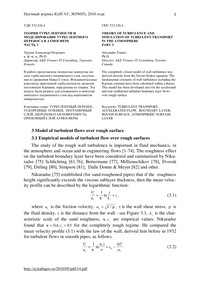
    Figure 3.2: The rough surface effect on the turbulent flow: 2D roughness elements data [88-105], the solid line is calculated on the model of Dalle Donne & Meyer [82]

    Figure 3.2 demonstrates D₁(Ad) calculated according to (3.6) - solid line (1) and the experimental data found for 2D roughness elements by various authors listed in Table 3.1 (the corrected and reduced data or R (да )₀₁ from Table 2 of Dalle Donne & Meyer [82] has been used as long as correlation (3.6) was proposed for this values).The symbols description is given in the right part of Figure 3.2 and Table 3.1. As Figure 3.2 shows the correlation is good for the middle and high value of the roughness density parameter, but for A*D «1 the scatter of the points is rather large and can't be explained by the experimental technique differences only. The empirical model [82] can't explain the experimental behaviour of the mean velocity shift with a roughness density, which can be found out only by comparison of large number of the data, obtained by various authors [75-77, 81-83, 87-109].
    Osaka & Mochizuki [110] examined d-type rough wall boundary layer in a transitionally and a fully rough regime. They have shown that in a transitionally rough regime the mean velocity logarithmic profile is confirmed and that the Karman constant has the same value as for the hydraulically smooth wall flow.
    The mean velocity logarithmic profile widely used in the atmospheric turbulence research is given by (see [18-20, 25, 111-113]):
U ¹, z - zd — = —ln-----ur К z 0
    where zd is the displacement height, z₀ is the roughness length. Note that zd and z₀ are considered often as some adjustment parameters chosen for the best correlation of the local wind profile in the neutral stratified flow with the logarithmic profile. The model of the displacement height has been considered by

http://ej.kubagro.ru/2010/05/pdf/14.pdf

Научный журнал КубГАУ, №59(05), 2010 года

7

Jackson [112]. The classification of the experimentally determined roughness length for various terrain types was given by Wieringa [113].
    3.2 Model of wall roughness effect on turbulent flow
    The effective wall location was defined by Schlichting [76] as the mean height of the roughness elements and in the mathematical form can be written as:

Az = rₐ

1
Ll

- JJ r ( x, y ) dxdy У AxAy

(3.7)

    where z = r(x,y)is the relief of the rough surface - see Figure 3.1, Lₓ,Ly are the rough wall scales in the x, y directions, AxAy = LₓLy.
    In a case of two dimensional roughness considered by Dvorak [79] and Simpson [81] the roughness density parameter depends on the width and pitch of roughness elements (see Figure 3.1): A s = L / d. The mean roughness height depends on the height of roughness elements as rₐ = akr / As, where a is the numerical constant which equals to unity in this case. Using the Bettermann-Dvorak's equation (3.5) in the rang 4.68 < As < 102 the shit of the mean velocity can be presented as a function of the mean roughness height, thus we have
— = Iln uk- + D - 2.5 lnuk- - 0.35ln As + 5.95 =
                  u к v                    v A s

ur
= 2.5ln~^- - 0.35ln A + 5.95 v                s

    In this approach the mean velocity profile in the turbulent flow over a rough surface can be rewritten as follows

                    U1z
                    — = —ln— + 0.35ln A - 0.45
                    Uy к rₐ

    If we redefined the main roughness scale then the mean velocity profile

takes the form which widely used in the atmosphere research:

U
uy

¹1 z1
= —ln—
к  r0

(3.8)

where lnr = lnr - 0.35кln A, + 0.45к - lnr - 0.14ln A, + 0.18 . Practically r - r 0               a           s            a         s                    0a
for A s = 5 and r0 - 0.6³ra for A s = 100. Hence, the logarithmic profile mainly depends on the mean height of the roughness elements in this range of the roughness density.
    Let us consider the random function defined as

http://ej.kubagro.ru/2010/05/pdf/14.pdf

Научный журнал КубГАУ, №59(05), 2010 года

8

uz₁
u(Z1 / r) = ln—
K r


(3.9)

    where r is the random parameter with the mean value given by

                                                         fw
                                                           ₀rfₛ(r)dr


     here fₛ = fₛ (r) is the density of a probability distribution function (roughness statistic function) normalised on unity:
                                     fw
,0 fs ⁽r)dr = 1
     Both parts of equation (3.9) can be averaged with this function as follows
                        w                   w
                                         u                      uz
U ⁽z1⁾ = J u⁽ z1 / r ⁾ fs ⁽r )dr = — J(lⁿ z1 - lⁿ r ) fs ⁽r ⁾ dr = ~ lⁿr
0                 K 0                  K r0

    where   lnr0 = J ln(r) f (r)dr . With this result the mean-squared-value of the
⁰0         s
velocity fluctuations can be calculated as w                                          w
Su = J⁽u ⁻ U)2fₛ⁽r)dr = J⁽lₙ r ⁻ ln r0⁾²fₛ ⁽r)dr
0               K 0
    Therefore we have

Su² = — (^ln² r - ln² r0)

    Thus, the random function u~(z₁/r)can be used for the mean velocity calculation as well as for the mean-squared-value of the velocity fluctuations modelling. Our main idea is that the random function u~(z₁/r) can be calculated on the basis of a solution of the Navier-Stokes equation due to the surface layer transformation

u⁽ zi / r) = Jim ~& Ju ⁽x, у , ^i^dxdydz
SV^dVs SV
S'r SV

(3.10)

    where ^ₗ = z1 / r(x,y) is fixed over the integrated region, = z 1 / r = const, SV
is an arbitrary volume put in dV = LxLydz and containing dVₛ as a whole, dVₛ is the subregion in which altitude of the rough surface r(x,y) varies in limits from r up to r + dr, hence by definition dVₛ = dVfₛ (r)dr .
    Note, that the surface layer transformation is only a kind of averaging procedure which conserves the function properties across a boundary layer. The Navier-Stokes equation can be averaged with the surface layer transformation (3.10) instead the normal Reynolds averaging method to derive then the equation for the random amplitude u~(z₁/r). Unfortunately it's impossible to use this

http://ej.kubagro.ru/2010/05/pdf/14.pdf

Научный журнал КубГАУ, №59(05), 2010 года

9

method in the simple form (3.10), because, for example, in the case of a smooth flat plate r = 0.
    Therefore we suppose that there is a surface z = h(x,y, t) (the dynamic roughness surface) inside the flow domain which can be used for modelling the rough surface effect on the turbulent flow. Without any limits we can choose a surface z = h (x, y, t) close to the wall surface z = r (x, y), but not equal to r (x, y).
    Let h(x,y,t) = r(x,y) + hᵣ(x,y,t), where hᵣ(x,y,t)is the height of the viscous sublayer   over  the  rough   surface.    In   the  turbulent  flow   the  surface
z = h(x, y, t) can be described by random continuous parameters h, ht, hx, hy characterised the height, velocity and inclination of the surface elements. Let’s define the subregion dVₛ in which the local height of the rough surface r(x,y) varies in limits from r up to r + dr and parameters of the surface z = h(x, y, t) in limits from h up to h + dh , from hₜ up to hₜ + dhₜ , from hₓ up to hₓ + dhₓ , from hy up to hy + dhy , thus

dVs = dVfₛ (r, h, hₓ, hy, hₜ)drdhdhₓdhydhₜ,
    where fₛ = fₛ (r, h, hₓ, hy, hₜ) is the multiple density of a probability distribution function. Therefore in common case the surface layer transformation can be written as follows (instead of eq. (2.1) or (3.10))
                                                 ¹
u(z 1 / h, t, r, h, h , hy, ht) = lim — I u(x, y, q, t)dxdydz s                     8V^dVs AV •>
SV
    where     ^ =  z 1/ h (x, y, t )is fixed over the    region   of   integration,
^ = z 1 / h = const, SV is an arbitrary volume put in dV = LₓLydz and containing dVₛ as a whole.
    Here again we have the starting point of the theory of turbulence explained in second chapter. On this way we have lost the simplicity of transformation (3.10), as there is an unknown dynamic roughness function h = h (x, y, t) in transformation (2.1).
The additive dynamic roughness surface model considered above is given by h ( x, y, t) = r ( x, y ) + hᵣ ( x, y, t)
    where hᵣ(x,y,t)is the height of the viscous sublayer over the rough surface. Averaged this equation over a large area AxAy = LₓLy we have: h = rₐ + hr, htₜ = hiᵣₜ, where rₐ is the mean roughness height, i.e.
ra = L~L~ Лr ⁽x, y) dxdy
AxAy

http://ej.kubagro.ru/2010/05/pdf/14.pdf

Научный журнал КубГАУ, №59(05), 2010 года

10

    After replacing of the origin of the coordinate system in the new position z ^ z - rₐ the dynamic roughness equation can be written as:

h1( X, y, t) = r ( x, y ) ⁻ rₐ + hᵣ ( x, y, t t)

(3.11)

    where   ht = hr, htₜ = hᵣₜ. Thus, we can imagine the smooth wall located at
z = rₐ as it was defined by Schlichting [76] and the dynamic roughness surface with the dynamic roughness parameters given by (3.11). For this problem we should suggest that ht > 0.
    Note that the fluid flow near the plate surface z = rₐ is a typical heterogeneous flow included two parts: the roughness rigid elements part Sₐ = Sₐ(rₐ) and the fluid flow part equals to ДS - Sₐ, where ДS = LXLy. Put Лₐ = ДS / Sₐ (rₐ) is the ratio of the whole area ДS = LXLy to the roughness area Sa = Sa (ra )at z = ra • The roughness density parameter proposed by Dvorak [79] is given by Лₛ = Д8 / S, where S is the total roughness area. Since rₐ = akr / Лₛ, so Лₐ = Лₐ (rₐ) can be considered as a function of the Dvorak's roughness parameter: Л ₐ = Л ₐ (Л ₛ). For the roughness elements considered by Bettermann [77], Schlichting [76] and Coleman et. al. [83] this function can be calculated in the closure form.
    For the roughness compounds by the spherical uniform elements rₐ = 2k„ /3Л, , Sa (rₐ) = S[1 - (1 - 2rₐ / k„)²], hence

t 8 f 2 ^
             — =--d t--I
             Л a 3Л 2 к 3Л , J
as     s

(3.t2,a)

    In the case of the surface roughened by spherical segments (Figure 3.t) we have: rₐ = kᵣ(3 + kᵣ² /r²)/6Л,, Sa(rₐ) = S(1 + rₐkᵣ /r²)(t-rₐ /kᵣ), therefore
'  S    )   '        V   e⁽ ³ ■ e⁾|      (3 12.
Лₐ ДS Лₛ        к¹ 6Лₛ Л¹ ⁺ 6Лₛ J        l ’

    where, e = kᵣ² / r².
    In the case of the surface with conical uniform elements we have
    S. (r.) = S (1 - r„ / k, )2 , r„ = kr/3Л s, thus

-L = -L ft - -L1 Л a Л s к¹ 3Л s J

(3.t2,c)

    In the case of two dimensional roughness as it has been considered by Bet-termann [77], Dvorak [79] and Dalle Donne & Meyer [82] Л ₐ = Л ₐ (rₐ) depends only on the roughness elements width and pitch (see Figure 3.t):
Лa =Лs = L / d                   (3.t2,d)

http://ej.kubagro.ru/20t0/05/pdf/t4.pdf