Политематический сетевой электронный научный журнал Кубанского государственного аграрного университета, 2010, №60

Научный журнал КубГАУ, №60(06), 2010 года 

http://ej.kubagro.ru/2010/06/pdf/31.pdf

1

УДК 532.526.4 
 
UDC 532.526.4 
 
ТЕОРИЯ ТУРБУЛЕНТНОСТИ И 
МОДЕЛИРОВАНИЕ ТУРБУЛЕНТНОГО 
ПЕРЕНОСА В АТМОСФЕРЕ  
ЧАСТЬ 6 

THEORY OF TURBULENCE AND 
SIMULATION OF TURBULENT TRANSPORT 
IN THE ATMOSPHERE  
PART 6  
  
Трунев Александр Петрович 
к. ф.-м. н., Ph.D. 
Alexander Trunev 
Ph.D. 
Директор, A&E Trounev IT Consulting, Торонто, 
Канада 
Director, A&E Trounev IT Consulting, Toronto,  
Canada  
 
Дана модель непрерывного перехода от ламинарного к турбулентному течению в пограничном 
слое. Развита теория спектральной плотности турбулентных пульсаций 

The model of continuous transition from the laminar 
flow to the turbulent flow is proposed and the theory 
of the spectral density of turbulent pulsation is given 

 
 
Ключевые слова: АТМОСФЕРНАЯ 
ТУРБУЛЕНТНОСТЬ, ТУРБУЛЕНТНЫЙ 
ПЕРЕНОС, УСКОРЕННЫЕ ТЕЧЕНИЯ,  
ПОГРАНИЧНЫЙ СЛОЙ, ШЕРОХОВАТАЯ 
ПОВЕРХНОСТЬ, ПРИЗЕМНЫЙ СЛОЙ 
АТМОСФЕРЫ, ТУРБУЛЕНТНЫЙ ПЕРЕНОС 
АЭРОЗОЛЕЙ 

Keywords: ACCELERATED FLOW,  AEROSOL 
TURBULENT TRANSPORT, ATMOSPHERIC  
STRATIFIED FLOW, ATMOSPHERIC 
TURBULENCE, ATMOSPHERIC SURFASE 
LAYER, BOUNDARY LAYER,  ROUGH 
SURFACE, TURBULENT TRANSPORT  

 

6. Dynamics of boundary layer 

6.1. Boundary layer structure 

During the last twenty years mathematical modeling of turbulent flows of 
fluid has been successfully developed in several directions at once [1, 19-54, 5970, 74-128]. Methods of direct numerical simulation (DNS) [66, 116], large 
eddy simulation (LES) [140], and different models, based on Navier-Stokes 
equations averaged according to Reynolds's method [28-38, 44, 51] have to do 
with these directions. The theory of hydrodynamic instabilities and transition to 
turbulence was proposed, which is based primary on the mathematical ideas 
about behavior of the dynamical systems [141-142]. The fractal geometry theory 
developed by Mandelbrot [143] has been used to explain the chaos and intermittence in the hydrodynamic turbulence [144-145]. To obtain the numerical solutions of applied multidimensional problems the effective numerical algorithms 
have been created [146-147]. 

The boundary layer is a typical self organized flow formed around any rigid 
body moving in the viscose fluid at high Reynolds number. To illustrate the 
common problems of the boundary layer theory let us consider the structure of 
the boundary layer on the flat plate in adverse pressure gradient - see figure 6.1. 
This flow includes the laminar boundary layer (1), the transition flow (2), the 
turbulent boundary layer (3) and the separated turbulent flow (4).   

The laminar boundary layer is a well predicted and sufficiently investigated 
flow. But this flow is not a stable at high Reynolds number, because it can be 
like an amplifier for the waves of small amplitude.  

Научный журнал КубГАУ, №60(06), 2010 года 

http://ej.kubagro.ru/2010/06/pdf/31.pdf

2

The transition layer has a complex structure considered by many authors [62, 
141, 145, 149-151]. As it was shown by Jigulev [149] and Betchov [150] this 
flow domain includes seven sub-regions: 

1) 
the laminar flow region in which the small disturbances are generated. This part of flow is considered often as a starting point of transition 
layer. The Reynolds number of initial point of transition layer is a very sensitive to the boundary conditions on the wall and in the outer flow. The estimated value of the Reynolds number of transition is  
5
0
10
4
/
Re
⋅
≈
=
ν
U
xtr
tr
 
and as high as 
6
10
4
Re
⋅
≈
tr
;  

2) 
the quasi-laminar flow region in which the amplitude of linear 
waves (called  the Tollmien-Schlichting waves) grows up to the critical value 

2
0
10
/
−
≅
U
U
δ
. The typical scale of this region is about 
H
x
2
10
≈
∆
, where  H  
is a local thickness of the boundary layer; 

3) 
the nonlinear critical layer where the interaction between waves and 
main flow leads to the new unstable state. The typical scale of this region can 
be estimated as 
H
x
10
≈
∆
; 

4) 
3D waves region with scale  
H
x ≈
∆
 . In this region initial twodimensional waves are transformed into three-dimensional waves; 

5) 
the region of the secondary instability in which the short length 
waves are generated. The typical scales of this zone are about 
H
x
1.0
≈
∆
,
1
0
10
/
−
≅
U
U
δ
 ; 

6) 
the 
Emmons 
sports 
region 
with 
typical 
scales 
H
x ≈
∆
, 

1
0
10
3
/
−
⋅
≅
U
U
δ
. In this part of flow the non-equilibrium process leads to the 
turbulent spectrum of velocity fluctuations; 

7) 
the initial region of the turbulent flow in which 
2
0
10
3
/
−
⋅
≅
U
U
δ
. 

The transition from the laminar flow to the turbulent flow is a very attractive 
phenomenon from the mathematical point of view. Really the initial laminar 
flow, which is not consisting of any chaotic waves, then suddenly transforms to 
the state with a chaotic behavior. This problem of transformation called "dynamical chaos" has been investigated by many authors (see for instance [142, 
145]).  

The theory of the "dynamical chaos" is based mostly on the analyses of the 
simplifier dynamical systems (Lorenz-like chaos) which can't be used directly 
for the boundary layer problem.  

The turbulent boundary layer is characterized by chaotic pulsation of the flow 
parameters. The surface which separates the turbulent stream from the outer 
flow looks like a rough surface. The thickness of the turbulent boundary layer in 
zero pressure gradient increases with a distance approximately as a power func

Научный журнал КубГАУ, №60(06), 2010 года 

http://ej.kubagro.ru/2010/06/pdf/31.pdf

3

tion
2.0
Re
37
.0
/
−
≈
x
x
H
, and the skin friction coefficient slowly decreases with the 
Reynolds number increasing as   
2.0
Re
059
.0
−
≈
x
fc
where 
ν
/
Re
0x
U
x =
 (see 
Schlichting  [61]).  

 

               

 

 
 

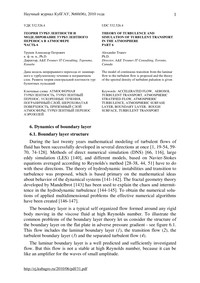
Figure 6.1: A) The boundary layer on the flat plate in adverse pressure 
gradient: 1 - laminar boundary layer; 2 - transition layer; 3 - turbulent boundary layer; 4 - turbulent separated flow; B) the thickness of the laminar boundary layer in the air flow at 
s
m
U
/
47
.
31
0 =
; C) the mean height of the separating boundary layer according to Simpson et al [148]      

  

The turbulent boundary layer in adverse pressure gradient separates out from 
the rigid surface and the boundary layer thickness increases as it is shown in 
Figure 6.1,c. This part of the boundary layer is not so well predictable as a laminar flow, thus till now the separated turbulent boundary layers were studied only 
in partial cases primary by experimental way (see Simpson et al [148]).   

The turbulent boundary layer can be modelled on the theory of turbulence 
which was explained in Chapter 2. But it is a very interesting fact that the laminar flow and transition layer also can be described by the equation system (2.14) 
derived from the Navier-Stokes equations (NSE) due to the special type of transformation (2.1). Let us consider the application of the turbulence theory to the 
quasi-laminar boundary layer, i.e. to the boundary layer flow which has some 
symptoms of turbulent flow.                

 

 

Научный журнал КубГАУ, №60(06), 2010 года 

http://ej.kubagro.ru/2010/06/pdf/31.pdf

4

 

6.2. Laminar boundary layer  

The general solution for the laminar flow can be found on the base of the 
boundary layer approximation of the Navier-Stokes equations in the Prandtl's 
form:  

2

2
1

0

z
u
x
p
z
u
w
x
u
u

z
w
x
u

∂
∂
=
∂
∂
+
∂
∂
+
∂
∂

=
∂
∂
+
∂
∂

ν
ρ

                                (6.1) 

Here the pressure gradient is given by equation (4.17), thus 

ρ
∂
∂

∂
∂
U
U
x
p
x
0
0 = −
.                                         (6.2) 

To derive model (6.1) from the Navier-Stokes equations we should suppose 
that  

a) 
the laminar boundary layer is a two-dimensional flow, i.e. 
)
,0,
(
)
,
(
w
u
z
x
=
= v
v
; 

b) 
the normal to the wall velocity gradient sufficiently exceeds the 
parallel to the wall velocity gradient, i.e. 
x
u
z
u
∂
∂
>>
∂
∂
/
/
; 

c) 
the normal to the wall pressure gradient is so small that it can be 
neglected, therefore the pressure distribution is described by the Bernoulli 
equation (6.2). 

It can be shown that the sufficient condition, to satisfy suppositions b)-c), is 
that the Reynolds number computed on the distance from the plate edge has an 
extremely high value, i.e.   
1
/
Re
0
>>
=
ν
xU
x
.  

 Boundary conditions for the quasi-linear diffusion equation (6.1) can be set 
as follows: 

 
)
(
)
,
(
:
,0
0
)
0,
(
)
0,
(
:
0
,0

)
0
(
)
,0
(
:
0
,0

0

0

x
U
z
x
u
z
x
x
w
x
u
z
x

U
z
u
z
x

→
∞
→
>
=
=
=
>

=
≥
=

                                                 (6.3) 

 

The first equation (6.1) can be satisfied automatically if we define a flow 
function as follows  

x
w
z
u
∂
∂
−
=
∂
∂
=
ψ
ψ
€
,
€
                                            (6.4) 

Problem (6.1)-(6.3) has a self-similarity solution for the boundary layer in a 
zero pressure gradient. In this case 
const
U
x
U
=
=
)
0
(
)
(
0
0
,  thus the first and third 

Научный журнал КубГАУ, №60(06), 2010 года 

http://ej.kubagro.ru/2010/06/pdf/31.pdf

5

condition (6.3) are identical that means that a solution of this problem depends 
on  the universal variable  
0
/
/
U
x
z
ν
η =
. Put 
)
(
€
0
η
ν
ψ
f
U
x
=
, then the velocity 
components can be rewritten as  functions of the universal variable, i.e., 

)
(
2
1
€
,
€
0
0
f
f
x
U
x
w
f
U
z
u
−
′
=
∂
∂
−
=
′
=
∂
∂
=
η
ν
ψ
ψ
                   (6.5) 

Substituting these expressions in the second equation (6.1) one can find that 
the universal function  
)
(η
f
 is described by the following equation (see, for example, [51, and 58]): 

0
2
=
′′
+
′′′
ff
f
                                              (6.6) 

The boundary conditions for equation (6.6) (these conditions can be derived 
from (6.3)) have a form 

1
)
(
,0
)
0
(
)
0
(
=
∞
′
=
′
=
f
f
f
                              (6.7) 

The problem (6.6-6.7) can be solved numerically using the algorithm described above in subsection 2.4.2. For the initial iteration one can put 
33206
.0
)
0
(
=
′′f
 (see [51]) that gives in practice the precise solution. Obviously 
that it's impossible to satisfy last condition (6.7) in a numerical procedure. 
Hence instead of it as usual the boundary condition in the outer region has used, 
9999
.0
)
(
=
′
e
f η
 where 
8
≈
e
η
 [51]. Thus the boundary layer depth can be defined 
as a point where, for instance, 
8
/
/
0 =
U
x
ze
ν
, i.e.  

0
/
)
(
U
x
x
H
ν
∝
                                    (6.8) 

This function is shown in Figure 6.1,b to illustrate the typical scale of laminar 
boundary layer in the air flow at  
s
m
U
/
47
.
31
0 =
. Therefore the universal variable 
can be presented as  
)
(
/
x
h
z
=
η
, where 
0
/
)
(
U
x
x
h
ν
=
 is the boundary layer characteristic thickness  

The boundary layer thickness is not a constant; it slowly increases down to 
the stream so that 

     
x
U
dx
dh
U
dt
dh
0
0
2
1
ν
=
=
                                        (6.9) 

 

This equation gives the normal to the wall velocity scale which can be defined as  
dt
dh
w
/
0 =
. With two characteristic scales of velocity equations (6.5) 
can be rewritten as follows: 

f
f
w
w
f
U
u
−
′
=
′
=
η
0
0
/
,
/
                                  (6.10) 

The normalised velocity profiles in the laminar boundary layer are shown in 
Figure 6.2. The normal to the wall velocity normalised on the scale 
dt
dh
w
/
0 =
 

Научный журнал КубГАУ, №60(06), 2010 года 

http://ej.kubagro.ru/2010/06/pdf/31.pdf

6

has a limit value at 
∞
→
η
: 
72
.1
/
0 =
w
w
. The positive value of this velocity component means that the stream lines starting from the boundary layer then penetrate in the outer flow region. 

 

 
 

Figure 6.2: The normalised velocity profiles in the laminar boundary layer 
in zero pressure gradient: 1 - 
0
/U
u
; 2 -  
0
/ w
w
 

 

The normal to the wall velocity scale decreases with distance as  

5.0
0
0
Re
5.0
−
=
x
U
w
. Thus near the transition layer this scale has a very small value 
which has never been taken into account in the theory of transition to turbulence.  

The skin friction coefficient can be defined for the laminar flow as 

x
f
f
U
z
u
c
Re
/)
0
(
2
)
2
/
/(
)
/
(
2
0
′′
=
∂
∂
= ν
. Substituted in this formula the numerical 
value of the second derivative,   
33206
.0
)
0
(
=
′′f
, which was calculated above, we 
have  
x
fc
Re
/
664
.0
=
. 

The self-similarity solutions (6.5) found for the laminar flow (called the 
Blasius flow) is only type of the self-similarity solutions of the Navier-Stokes 
equations (NSE). Let us give a proof that the Blasius flow can be described by 
equation system (2.14). Really all solutions of the equation system (2.14) which 
was derived from NSE are presented by the self-similarity functions. Therefore, 
we can select from (2.14) also solution for the Blasius flow. First of all note that 
in this two-dimensional flow   
0
v =
−
=
Ψ
x
y
h
u
h
,  and 
u
hx
=
Φ
, hence we have 

       

0

~

=
+
u
h
W

x
η
∂
∂
                                          (6.11) 

2

2
2
2
2
2

2
~

)
1(

~
~

η
η
η
ν
η
∂
∂
+
∂
∂
=
∂
∂
W
n
h
W
h
W
, 

Научный журнал КубГАУ, №60(06), 2010 года 

http://ej.kubagro.ru/2010/06/pdf/31.pdf

7

Here 
η
u
h
w
W
x
−
=
~
. Let  
)
(
~

0
η
f
h
U
W
x
−
=
, then the generalised form of  (6.5)  
and (6.6) can be found from first eq. (6.11) and from the definition of W~  immediately as follows    

)
(
,
0
0
f
f
U
h
w
f
U
u
x
−
′
=
′
=
η
                                 (6.12) 

0
)
1(
2

2
2
2

0
2

2
=
∂
∂
+
∂
∂
+
∂
∂
η
η
η
ν
η
f
h
U
hh
f
f
x
x
. 

The Blasius solution corresponds to the special case when  

2
)
/(
0 =
U
hhx
ν
,  
0
/
)
(
U
x
x
h
ν
=
.                            (6.13) 

In this case the second eq. (6.12) has a form  

 

0
)
Re
4
/
1(
2
2

2
2
2

2
=
∂
∂
+
∂
∂
+
∂
∂
η
η
η
η
f
f
f
x
                              (6.14)     

The boundary layer approximation (6.1) is applicable only for very high 
Reynolds number, i.e. for 
1
/
Re
0
>>
=
ν
xU
x
. Hence the term in the brackets 
which is proportional to 
x
Re
/
1
 can be neglected in (6.14) and finally we have 
equation (6.6).  

6.3. Transition to turbulence  

6.3.1. Continuous transition to turbulence  

Passing through the transition layer the laminar stream transforms into the 
turbulent flow. There are several models of transition to turbulence (see  [58, 
141, 145, 149] and other). From the point of view of the turbulence theory considered above the parameter characterized the dynamical roughness structure, 
i.e. 
)
/
arctan(
x
y h
h
=
α
, increases in the transition layer from a zero up to 
2
/
π
α =
, 

and the second turbulent velocity scale, 
2
2
*
0
/
y
x
t
h
h
u
h
w
+
=
+
, increases from a zero 

up to  
14
.0
0 ≈
+
w
. Consequently the 2D laminar Blasius flow transforms into 3D 
turbulent flow.  

The general solution (2.16) of the turbulent incompressible flow model (2.14) 
can be used to analyze the transition from the Blasius flow to the turbulent flow.  
Put  
)
0
(
),
0
(
2
1
η
η
u
h
A
u
h
A
y
x
=
=
 in this solution then the random velocity components 
can be written as follows 

+
+
+
=
−

2
2

2

2
2

2

1

sin
1
cos
)
0
(
~

η

α
η
α
η
η
n
n
e
u
d
u
d
I
,                               (6.15) 

+
−
+
=
−

2
2
2
2
1

1
1
1
2
sin
)
0
(
2
1
v~

η
η
α
η
η
n
n
e
u
d
d
I
,      

Научный журнал КубГАУ, №60(06), 2010 года 

http://ej.kubagro.ru/2010/06/pdf/31.pdf

8

2
2
1
cos
)
0
(
~

η
α
η
η

η
n
e
n
u
d
w
d
I

+
=

−
 

where  
∫
+
−
=
η

η
η
ν
2
2
1

~

n
d
W
h
I
.   

Put 
)
(
~

0
η
f
U
h
W
x
−
=
 as in the case of the Blasius flow then we have  

∫
+
=
η

η
η

ν
0
2
2
0
1
n
d
f
hh
U
I
x
                                        (6.16) 

where a function 
)
(η
f
f =
 satisfies to equation  

0
)
1(
2

2
2
2

0
2

2
=
∂
∂
+
∂
∂
+
∂
∂
η
η
η
ν
η
f
n
U
hh
f
f

x
                            (6.17) 

with  boundary conditions  

0
0
/)
0
(
)
0
(
,
/
)
0
(
,0
)
0
(
U
u
f
h
U
h
f
f
x
t
η
=
′′
=
′
=
.                   (6.18) 

Put  
2
)
/(
0 =
U
hhx
ν
 in (6.17) as for the Blasius flow solution, therefore    

                          
)
,
(
/
)
,
,
(
0
y
t
Q
U
x
t
y
x
h
+
= ν
,                            (6.19) 

where 
)
,
( y
t
Q
 is an arbitrary function.  

 

6.3.2.  3D Transition to turbulence 

The first scenario of spatial continuous transition to turbulence is that  
0
=
th
 
and 
33206
.0
)
0
(
=
′′f
. In this case the boundary conditions (6.18) are similar to the 
Blasius flow conditions. For 
0
=
yh
  we have exactly the Blasius flow solution - 
see Figure 6.3. Put 
0
/U
x
Q
ν
<<
 then the dynamical roughness parameters are 
given by  

2
2
Re
4
/
1
y
x
h
n
+
≈
,     
)
Re
2
arctan(
x
yh
=
α
.                        (6.20) 

 

As it follows from this equations if 
yh  increases then the dynamical roughness parameters also increase and the laminar boundary layer velocity profile 
(the Blasius profile (1) in Figure 6.3) transforms into the turbulent boundary 
layer velocity profile (6) - see Figure 6.3.  

Научный журнал КубГАУ, №60(06), 2010 года 

http://ej.kubagro.ru/2010/06/pdf/31.pdf

9

 
 

Figure 6.3: Continuous transition from the laminar flow (the Blasius velocity profile (1)) to the turbulent flow (the logarithmic velocity profile (6)). 
Profiles 1-6 
are 
computed 
on 
(6.17)-(6.18) 
for 
0
=
th
 
and 
for 

2
;3
/
4
;1
;3
/
2
;3
/
1
;0
=
yh
 respectively 

 

 
Figure 6.4: Continuos transition to turbulence: 1 - the mean velocity profile in the turbulent boundary layer according to Van Driest [65],  2, 3 - the 
mean velocity profiles in the transition layer computed on the model (6.24), 
(6.25) for   
5.3
,
91
.0
=
yh
 respectively 

 

Theoretically the logarithmic profile in this model can be only at 
∞
→
n
, but 
practically the logarithmic asymptotic is realised for 
5.3
=
n
 - see Figure 6.4.   It 
can be explained by the asymptotic behavior of a solution of equation (6.17) at 

∞
→
η
: 
)
(
)
(
)
(
n
n
f
β
η
γ
η
−
≈
, where 
)
(
),
(
n
n γ
β
 are some parameters. Obviously, 
that for the Blasius flow 
1
)
0
(
,
72
.1
/)
(
)
0
(
0
=
=
∞
=
γ
β
w
w
, and in a common case 

n
n
2
/1
)
(
≈
β
 for 
1
≥
n
. Therefore 
)
(η
I
 can be estimated for 
∞
→
η
 as follows 

)
1
ln(
4
)
(
1
2
1
2
2
2
0
0
2
2
η
γ
η
η
η
n
n
n
I
n
d
f
I
+
+
=
+
= ∫
                               (6.21) 

Научный журнал КубГАУ, №60(06), 2010 года 

http://ej.kubagro.ru/2010/06/pdf/31.pdf

10

∫

∞

+
−
=
0
2
2
0
1
)
(
2
1
η

η
γη
n
d
f
I
. 

Substituted this expression in the first equation (6.15) and supposed that 
2
/
π
α =
 one can derive the asymptotic formula for the streamwise velocity gradient, i.e.   

1
,
)
(
)
0
(
~
0
>>
≈
−
−
η
η
η
η

η
n
n
n
e
u
d
u
d
b
I
                                 (6.22) 

Here 
3
2
4
/
1
2
/
n
n
b
≈
= γ
 for 
1
≥
n
. Used the inner layer variables for the mean 
velocity scaling the last equation can be rewritten as follows 

b
I

z
z
e
dz
du
≈
+

+

+

−
+

+

+
λ
λ
0
.                                         (6.23) 

Calculated the exponent b  for 
5.3
=
n
we have 
006
.0
≈
b
. Thus in this case the 
power function factor in the right part of equation (6.23) is about unit for 

3
3
10
/
10
≤
≤
−
λ
z
 hence equation (6.23) leads to the logarithmic profile asymptotic 

+
+

+
≈
z
dz
du
κ
1
 

Here 
+
=
λ
κ
/
0Ie
 is the Karman constant. Using the relationship 
κ
λ
/
0
Ie
=
+
  
third boundary condition (6.18) in a case of mean velocity profile can be transformed as follows 

+
+
+
+
+
+
+
=
=
=
=
′′
0
0
0
0
/
/
/
)
/
(
/)
0
(
)
0
(
0
U
ne
U
n
U
h
dz
du
U
u
f
I
κ
λ
η
 

Using the inner layer variables we can rewrite the model of spatial transition 
to turbulence in the form       

+
+
+
=
+
+
+
+
−
+

+

2

2

2

2

)
/
(
1

sin
)
/
(
1
cos

λ

α
λ
α

z
z
e
dz
du
I
 ,                       (6.24) 

0
)
1(
2

2
2
2
2

2
=
∂
∂
+
∂
∂
+
∂
∂
η
η
η
η
f
n
f
Rf
,  
∫ +
=

η

η
η

0
2
2
1
n
d
f
R
I
, 

∫

∞

+
−
=
0
2
2
0
1
)
(
η

η
γη
n
d
f
R
I
, 
η
η
γ
η
/)
(
lim f
∞
→
=
, 

where  
)
Re
2
arctan(
x
yh
=
α
, 
2
2
Re
4
/
1
y
x
h
n
+
≈
, 
,
/
+
+
=
h
z
η
 
2
/
1
/
0
=
=
ν
U
hh
R
x
 (as 
for the Blasius flow), 
+
+ = λ
n
h
, 
κ
λ
/
0
Ie
=
+
. The boundary conditions for this 
model are given by 

 
+
+
=
′′
=
′
=
=
0
/
)
0
(
,0
)
0
(
,0
)
0
(
,0
)
0
(
0
U
ne
f
f
f
u
I
κ
                      (6.25)  

The mean velocity profiles computed on the model (6.24) for  
5.3
,
91
.0
=
yh
 
(the solid lines 2,3) together with the mean velocity profile in the turbulent